HOW TO USE VLOOKUP IN EXCEL-EASY EXAMPLE
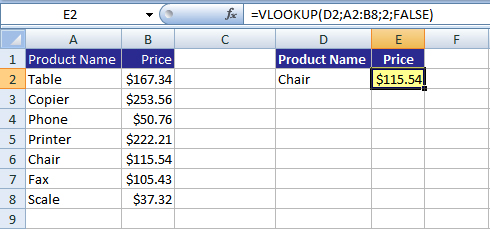
Below is the anatomy of the Vlookup function in Excel. In this article, we clearly explain VLOOKUP with a simple example and the elements of VLOOKUP including LOOKUP_VALUE, TABLE_ARRAY, COL_INDEX_NUM, AND RANGE_LOOKUP. In this example, we will be using the formula: =vlookup(D2;A2:B8;2;FALSE).
LOOKUP_VALUE |
| The lookup_value is the value that you have in one part of your document, whose corresponding value you want to find in another part of your document. |
| EXAMPLE: |
| You might have a product name in one part of your document, and you want to find its corresponding price in another part of your document. In the example below, the Lookup_Value is “Chair” in cell D2. We will want to look up the word “Chair” in the range A2:B8, find the value that is next to Chair, which is $115.54, and place it into cell E2 next to the word “Chair”. To get $115.54 in cell E2, the formula that we will enter into that cell is =vlookup(D2;A2:B8;2;FALSE). In this formula, D2 is the Lookup_Value. |
| NOTE: The lookup_value can be a value (such as number, text, or logical value) or it can be a reference such as A2. |
TABLE_ARRAY |
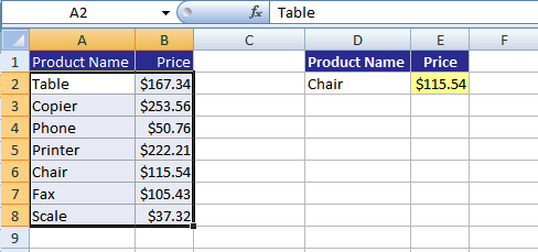
| You set the table_array range to specify the range of cells that you want Excel to look thru to find the value you are looking for and then to find it’s corresponding value. In the example we used above, in the formula =vlookup(D2;A2:B8;2;FALSE), the table_array is A2:B8. The image below, shows the table_array selected. |
| IMPORTANT NOTE: The lookup_value you are looking for in the table_array range should be in the first column of the table_array range. In this example, our lookup_value is “Chair” and it is in the first column (column A) of the table array_range of A2:B8. |
| NOTE: If you use an absolute reference ($A$2:$B$8), instead of a relative reference (A2:B8), it will be easier to copy the formula to other cells. Or else, name the lookup table, and refer to it by name. |
COL_INDEX_NUM |
| Within the table_array range that you specified, which column do you want Excel to look thru to find the corresponding value that you want returned? |
| In the example above, the table_array range is (A2:B8), and you want Excel to return a value from column B of that range (you want Excel to return $115.54 into cell E2), so your col_index_num would be 2 because Column B is the second column in the range A2:B8. |
| 1) If col_index_num is less than 1, VLOOKUP returns the #VALUE error. |
| (this is because you must specify at least one column) |
| 2) If col_index_num is greater than the no. of columns in table_array, VLOOKUP returns the #REF! error. |
| (this is because you can’t use a column no. more than the no. of columns you have.) |
RANGE_LOOKUP |
| Range_lookup specifies whether you want an exact or approximate match returned. |
| In our example, in the formula =vlookup(D2;A2:B8;2;FALSE), we used FALSE to get an exact match. |
| 1) If you use TRUE for Range_lookup: |
| ● (TRUE is most often used to find numeric data) |
| ● An exact or approximate match can be returned. |
| ● Sort the first column of the table_array in ascending order, otherwise you may not get the results you want. |
| 2) If you don’t use Range_lookup: |
| ● (This is most often used to find numeric data) |
| ● An exact or approximate match can be returned. |
| ● Sort the first column of the table_array in ascending order, otherwise you may not get the results you want. |
| 3) If you use FALSE for Range_lookup: |
| ● (FALSE is most often needed when looking for a text match) |
| ● Excel will look for an exact match only. |
| ● The values in the first column of the table_array do not need to be sorted. |
| ● If there are two or more values in the first column of the table_array that match the lookup_value, the first value found is used. |
| ● If an exact match is not found, the #N/A error is returned. |


 Hi, I am Suzanna. Thanks for visiting!
Speak Your Mind